Table of Contents Show
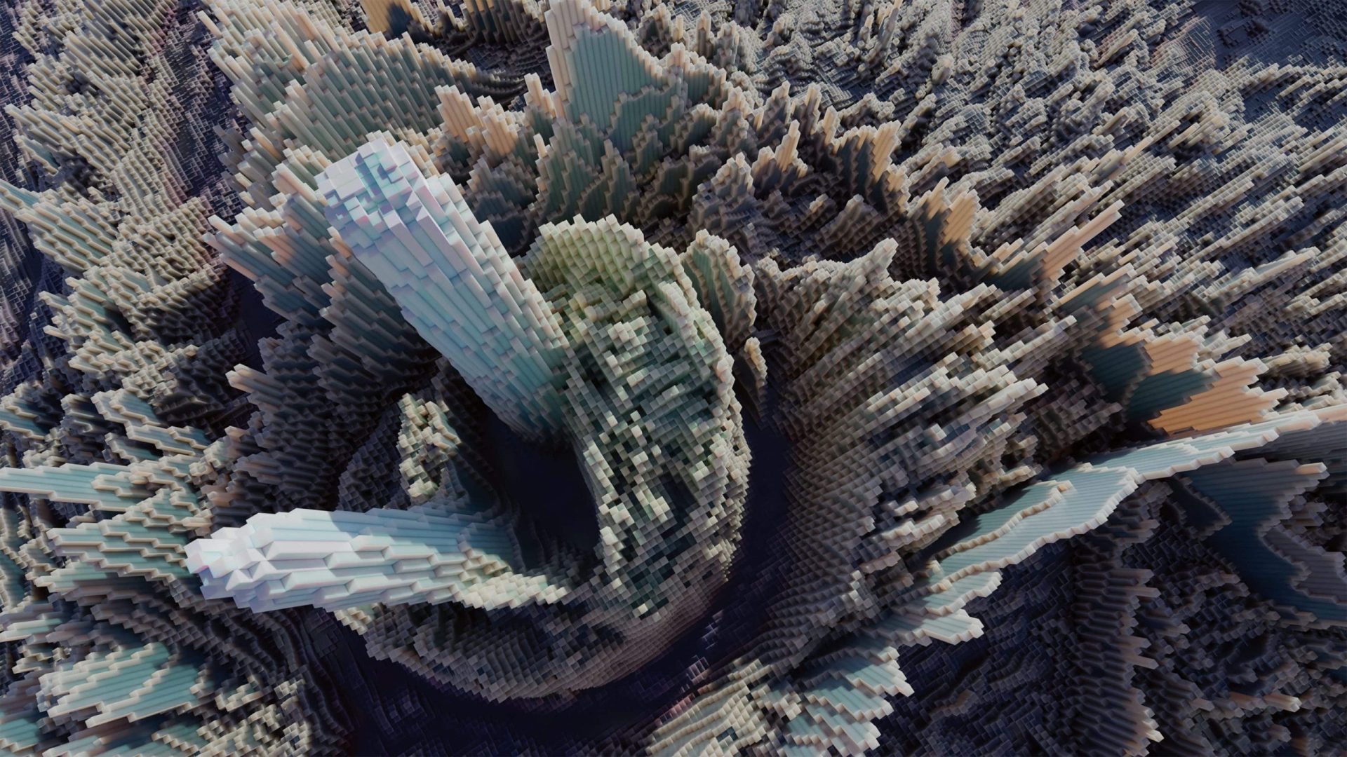
The best way to do this is to use newly added nodes to get to know Blender 3.5 a little better. In this workshop, we will create a Geometry Nodes setup that can be used to automatically generate landscapes like these from images, which are abstractly reminiscent of skyscrapers.
New in Blender 3.5 – The Image Info Node
The effect to be created in this workshop is also possible with older Blender versions. In Blender 3.5, however, a node has been added that makes it easier to make adjustments, namely the “Image Info” node. With this node, our result is really round and something that can be called an asset. This is because this node can be used to read out the size of an image in pixels. Not only can this information be used to place and colour a block on exactly one pixel of the image, it can also be used to calculate the correct aspect ratio and guarantee that the blocks are always exactly the same size, regardless of how many or few pixels the original image has.

Cat Content
In our case, the source image should be a cat portrait that can be downloaded from is.gd/blender_cat . However, you can use any image you like. In general, high-contrast images are particularly suitable; in addition to cat content, satellite images are also often used for this effect, probably because of the visual proximity of the result to city shots taken from an aeroplane.
Our asset
The finished asset will be inserted by the application like an object using drag-and-drop. It will receive an image and various parameters as input. So that the user immediately has something to look at, it comes with a sample image and is also provided with a material. A cuboid is placed at each pixel of the original image, which takes on the colour of that pixel.
Variable size or variable pixel density?
You could build the asset in such a way that the size of the object along an axis always remains the same, regardless of how high or low the resolution of the image is. However, as there are images with different aspect ratios, we would not have gained much from this, as without distortions the size along an axis must remain variable. If, on the other hand, we take the length and width of the cuboids that appear at each pixel as a fixed parameter, the size of the overall object can change along two axes depending on the image, but the rods do not become thinner or thicker.

The default cube can remain
Even if the asset can later be inserted into the scene as a separate object, it needs a start object for the first iteration. The default cube will be used for this, which for once will not be deleted immediately. Instead, go to the Geometry Nodes workspace by clicking on the corresponding tab in the header. The 3D viewport is now noticeably smaller and most of the space is taken up by a node editor in the lower area, where you can create a new node tree using New. It is best to give it a descriptive name such as “Image to Skyscrapers”.
Everything stays the same
The node tree does not yet make any changes to the cube, there is only one node group input and one group output. These two nodes control our inputs, i.e. the data with which the node setup is fed, and our outputs, which can be pure geometry as well as additional data that we can access in a shader, for example.
New in Blender 3.5


Now add an image info node using Shift A. This is a new addition in Blender 3.5 and can be found under Input – Scene. This node can be used to request information about an image opened in Blender, including the width and height, which we will need later. To load an image, you can click on Open or insert an image into the purple input socket. In our example, we will later use another node that receives an image from input. It therefore makes sense not to load the image in both nodes separately, but to load it further up in the node tree and then feed it to both nodes. It would be even better from the user’s point of view if the image could be selected outside the node tree. To do this, draw a connection from the purple input socket of the image info node to the empty circle output socket of the group input node.
Our own modifier
A new Image field has now appeared in the Geometry Nodes modifier on the right-hand side of the Properties Editor in the Modifier Properties tab with the blue spanner. We use Geometry Nodes to create our own modifiers, which are fully integrated in the stack and are also controlled from there. Specifically, we define what comes out of the outputs of the group input node, in our case so far the image that we use for the effect. A clear arrangement as well as suitable names and an optional description are mandatory here so that the asset can later be used intuitively by other users. Of course, you also benefit when you take it out again after months and have to find your way around.
Best practices
Click on the Group input node and open the sidebar using the N key or by clicking on the tiny < in the top right-hand corner of the Node Editor. There, in the Group tab, you can change the order of the sockets of the Group Input and Group Output node, add and remove new sockets, change their data type and specify a name, a tooltip and a default value.
Misuse
The interface still has one small disadvantage: in the selection field for the image, you can only select those that are already loaded as a datablock in Blender. The icon for opening the Blender file browser, which is usually used in other fields for selecting images, is missing. This means that you have to load your desired image elsewhere, for example in a Blender image editor. At this point, it is a good idea to turn the Spreadsheet Editor at the top left of the Geometry Nodes workspace into an image editor, load the desired image and then select it in the field in the Geometry Nodes modifier.
Viewport
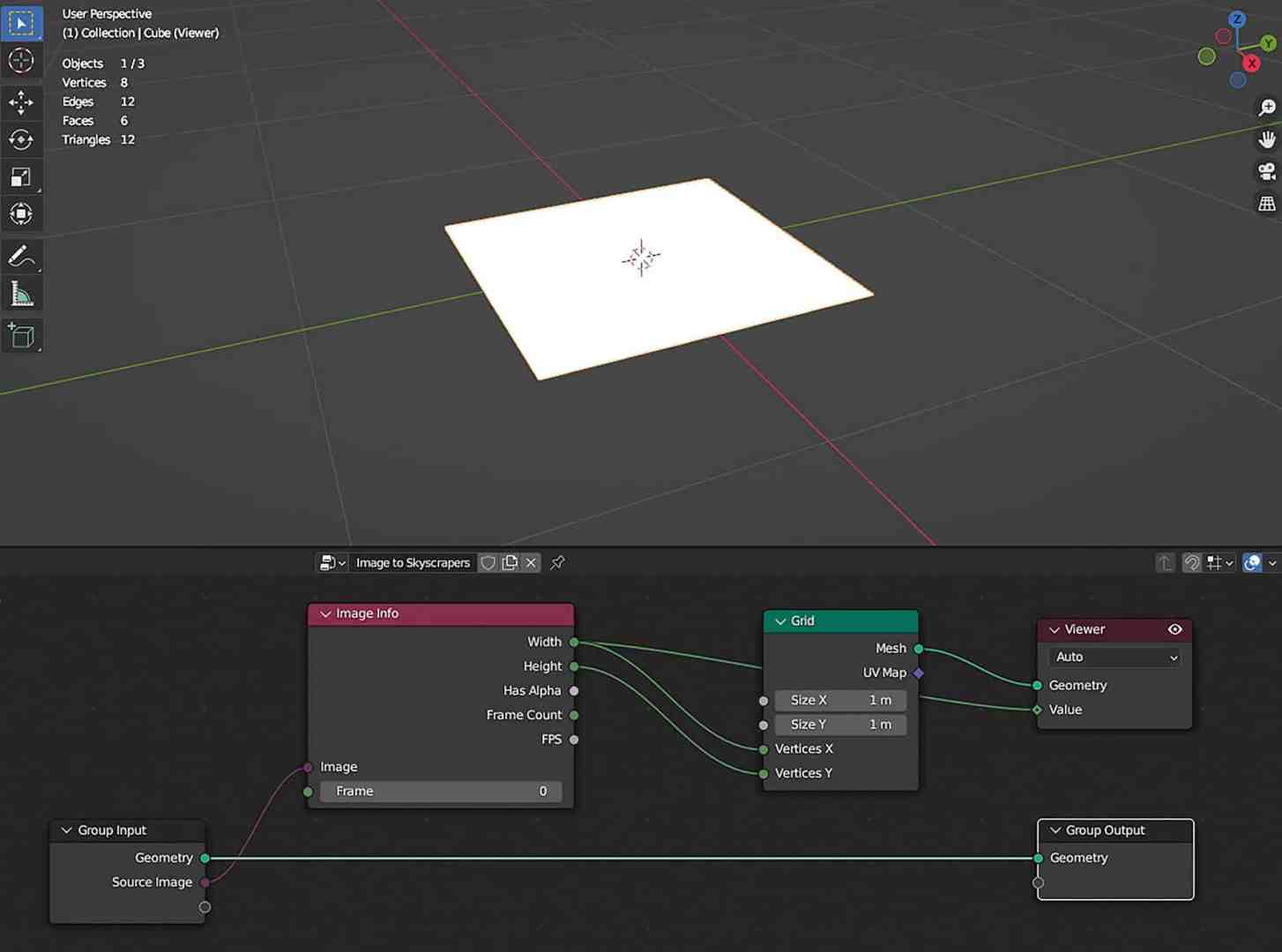
We have now reached a point where we can view the first data in the Node Editor, specifically the width and height of the input image. However, these are not displayed directly on the socket, which must first be evaluated, or in other words: We have to put something in, then we can find out the value. This is what the Viewer Node is for. Hold down the CTRL-Shift key and click on the image info node. A viewer node appears that is directly connected to the top socket. In addition, the cube has disappeared in the 3D viewport, because what is fed into the viewer node is now displayed there. And the geometry socket is currently empty, but there is a socket value directly below it. Move the mouse over it and the value appears with the data type in brackets in a tooltip, in the case of the cat image this would be 1536 Integer. You can already work with this.
Grid
If we later want to place an object at all pixels of the image, we need points. And these can be taken very easily from a mesh using Geometry Nodes. Add a grid node via Mesh – Primitives and connect Vertices X with Width and Vertices Y with Height. Continue to connect the mesh output with the geometry input of the viewer node and a plane becomes visible in the 3D viewport. We now see the input of the viewer node and no longer the normal result of the geometry nodes. You can see that this is only a view and not the actual scene if you switch on the statistics in the overlays. The eight vertices of the cube are still displayed there, whereas there should actually be many more in the grid. If you click on the eye symbol at the top right of the viewer node, it is deactivated and the cube appears again. If you connect the mesh output of the grid node to the geometry input of the group output node, the layer appears in the viewport again, but this time the statistics show the correct number of vertices. The viewer node is very useful for displaying intermediate results. It is no longer needed at this point, delete it with the X key.

Aspect ratio
The grid is square, although the number of vertices in X and Y are different. This is because the dimensions are defined by Size X and Size Y, both of which are currently set to one metre. Here again, it makes sense to influence the width and height of the image so that the aspect ratio is correct. There are various ways to proceed here. For example, you could define the object so that the length along one axis is fixed (e.g. always one metre along X) and the other axis is adjusted. Or the size of a pixel is fixed and the object can grow and shrink along both axes. The latter option is more suitable for this project, as the thickness of the individual pens remains the same. This allows us to use subsurface scattering later in the shader and the look remains the same, regardless of the image.
Maths
Add a Utilities > Math > Math Node and select Multiply from the drop-down menu. Connect the upper Value input socket to the Width socket of the Image Info node and the Value output socket to Size X at Grid. The strip is now extremely wide. Set the lower value of Value to 0.01 and draw a connection to the empty circle at Group Input. This has now also become an input field in the modifier. Call it “Pixel Size”. Because you first set the value in the field and then established the connection to the Group Input node, this value is now also the default value. The Math Node is now called Multiply in the header, as the currently selected operation is always displayed there. Duplicate it with Shift D and now also connect Pixel Size of Group Input to the lower input socket and Height of the Image Info Node to the upper one. Connect the result to Size Y of the grid node.
Our first asset
Basically, you now already have a practical asset. Namely a plane whose aspect ratio automatically adjusts to the selected image. If you use the same image as a texture, you won’t have any distortions. Of course, it would make sense to set the vertices in X and Y to a fixed value such as the default of three. Right-click on the cube in the outliner and select Mark as Asset and give it a descriptive name. Then save a copy of the file with File – Save Copy in your personal asset folder. Then connect Width and Height with Vertices X and Vertices Y again.
Cuboid ahoy
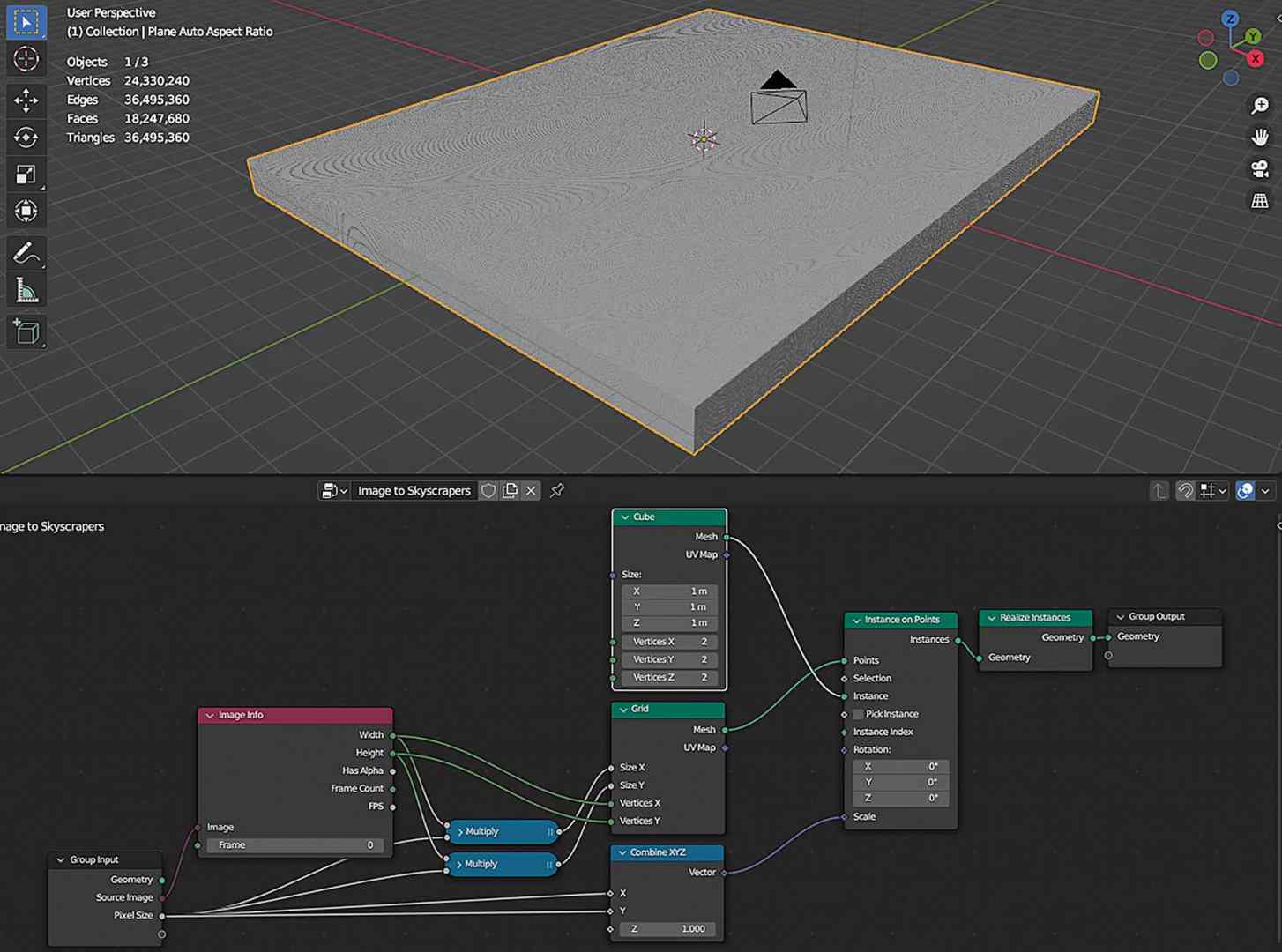
The next step is to build the small cuboids that will later create the abstract landscape. To do this, place a cube at each vertex or point of the grid and drag it out. Add a Node Instances > Instance on Points and place it on the connection between the grid and Group Output. The connection is created automatically, but the plane has disappeared in the viewport. This is because nothing is instantiated yet.
Click on the instance socket and drag out a connection. At the end you will see a symbol. This means that if you release the mouse over a free space, a search field will appear. Enter “Cube” there and after a short wait, millions of cubes will appear in the viewport. Although these are instances, Blender should now be almost impossible to use. This is because Blender has its problems with millions of objects, even if they are instances. Insert an Instances > Realise Instances node between Instance on Points and Group Output. Now the result is a whole object that consists of millions of vertices, but does not bring the viewport or the node editor to its knees.
millions of small ones.
Close together
To prevent the cubes from overlapping, the scale of the instances at X and Y should correspond to the pixel size. The Instance on Points node has a Scale input at the bottom, which is currently displayed as a square with a dot in the centre. This indicates that the scaling is applied individually for each instance and that different instances could also be treated differently. We will reserve the latter for the Z-axis, whose value we extract from the image.
However, the X and Y axes should directly adopt the pixel size. Drag a connection from the scale socket with the mouse and search for Combine XYZ. With this node you can freely configure vectors and the scale is such a vector. Connect X and Y with the pixel size from the group input node and initially set Z to 1.0. Now the object consists of millions of densely packed matchsticks, all of which still have the same height. But not for long.
Image height
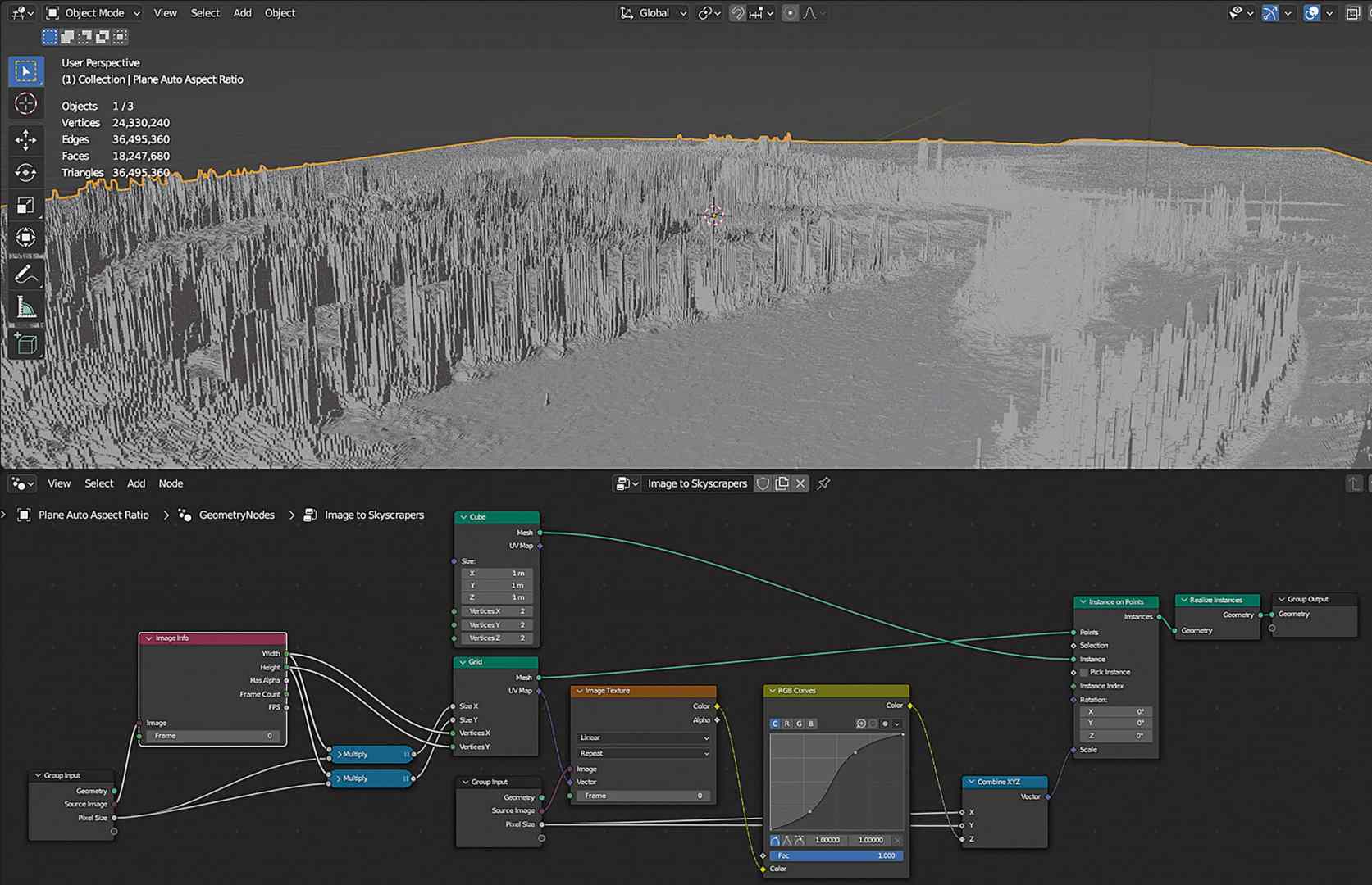
The height of the individual bars is to be extracted from the image. Conveniently, our grid has an output for the UV map. Add a Node Texture > Image Texture and connect the vector input to the UV map socket of the grid node. Add another Group input node via Input > Group. This is purely cosmetic, you can add as many group input nodes as you like. This prevents overlong node connections or noodles. You can take advantage of this by reconnecting the Pixel Size to the X and Y inputs of the Combine XYZ node.
Adjustment
The question remains as to how best to convert the colour information of the pixels into the height of the cuboids. Connect the colour output of the Image Texture Node to the Z input of the Combine XYZ Node. Blender now automatically converts the colour values of the texture into grey levels, which in turn determine the height of the cuboids. The nice thing about this is that we now have the usual colour manipulation tools at our disposal for fine-tuning. These can be found under Utilities > Colour. Add an RGB Curves node and adjust the contrast until you like the result. If you draw the typical S-curve, the smooth areas in the image will become even smoother and the peaks even sharper.
The colour must match the shader
The landscape already looks impressive, but the colour is still missing. This is only evaluated and displayed in the shader. The easy way would be to use the same texture again and map it correctly onto the blocks. However, this complicates the operation of the finished asset, as the user has to replace the image in two places. Alternatively, the colour information can also be transferred from the geometry nodes to Cycles, e.g. by storing it in the vertices of the output object
Output object. Then the user only has to select the image at one point and it becomes easier to replace the cuboids with other objects later, for example pins.

editor.
Material question
Two things are needed so that the colour of cycles can be read out. Firstly, we need to assign a material to the mesh. This will later become part of the asset. Secondly, we need to save the colour information in the mesh in order to be able to display it externally. Create a new material and add a Material > Set material node. Attach this between the cube node and the instance on points node and select the newly created material there.
Pick up
We can obtain the colour for each individual point on the grid via the image texture node, as we use the UV map of the grid for this. Later, however, these points disappear again and are replaced by instances of the cube. We therefore need to capture them first.
Add an Attributes > Capture Attribute node and place it on the connection between the grid and the instance on points. Select Colour from the drop-down above. A yellow colour socket now appears, which is evaluated individually for each point. Connect it to the colour output of the image texture node. We have now tapped the colour, but how does it get out of the geometry nodes and into the shader? To do this, connect the attribute output of the capture attribute node to the empty circle of the group output node. A new field has now appeared in the modifier under Output Properties.
You can change the name via the sidebar in the same way as for the Group Inputs. The name that we need later in the material is the name that you write in the field, e.g. StickColor. As soon as you enter a name there, the attribute is automatically created and also appears immediately in the Spreadsheet Editor.
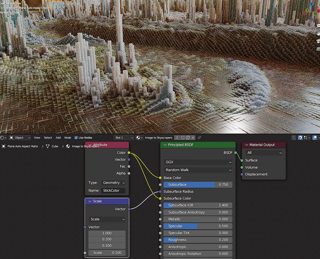
The lighting here comes from an HDRI from Polyhaven.
Bring in
Now we just have to get the colour into the shader or material. To do this, switch to the Shading Workspace and load the material into the Shader Editor. Add an Input > Attribute node and connect its colour output with Base Color and Subsurface Color of the Principled BSDF node. The last step is to copy the name from the field in the modifier and enter it in the attribute node. The sticks should now be coloured and the goal achieved.
Look
To achieve the look as in the hanger image, change the render engine to Cycles and set Subsurface to 0.75. To easily edit the subsurface radius, drag a connection from the socket and search for Vector Math Scale. Enter the values 1.0 0.2 and 0.1 for Vector. However, as the rods only have a width of 0.01, reduce the scale. You can experiment a little here, we decided on the value 0.075, smaller values make the result look redder and therefore fleshier. In the Principled BSDF, we have opted for a value of 0.2. The scene is illuminated by an HDRI from Polyhaven.
Tweaking
Our asset is actually finished in terms of the effect. You can now work with it and think about which other properties of the asset you want to control from the outside. For example, a multiplier for the height of the buildings or rods would be practical. To do this, add a Utilities > Math > Math Node between RGB Curves and Combine XYZ in the Geometry Nodes setup and set this to Multiply. You can now use the lower value for Value to determine the maximum height of the towers. First set this to 1.0 so that this value becomes the default value later and connect the socket to the empty circle at Group Input. Give the socket in the sidebar the name Max Height. We found a value of 1.5 very aesthetically pleasing for the demo image.

Finalising the asset
If not already done, mark the object with the Geometry Nodes modifier as an asset by right-clicking – Mark as Asset. Change an available editor window to an Asset Browser and select Current File from the dropdown in the top left. An asset should now appear with a grey layer as a preview. You can replace this preview with a file of your choice by opening the sidebar and clicking on the folder icon under Preview. Render at this point, save the result and select it as the preview image. Now you have a complete asset. If you save the file in your personal asset folder, you can always access it from now on via the Asset Browser as part of your personal library.
Conclusion
With Geometry Nodes and the Asset Manager, Blender has finally reached the point where you can create and package your own tools without programming knowledge, so that you can not only reuse them, but also distribute them to others. This workshop has shown the workflow of an asset creation with Geometry Nodes. The result can easily be dragged into existing Blender scenes via the Asset Browser. The result looks different depending on which image you load into it, but the thickness of the blocks and therefore the characteristics of the subsurface scattering effect remain constant. The resulting worlds invite you to linger and discover.


