Table of Contents Show
The script
After all the theoretical considerations, it is now time for the complete script.
// Initial variables
float g = 9.81; // Gravitational acceleration in m/s^2
float radius_p = 0.005; // Particle radius in m
float radius_p_var = 0.002; // Particle variance in m
float rho_p = 1050.0; // Particle density in kg/m^3
float rho_p_var = 30.0; // Particle density variance in kg/m^3
float rho_f = 1030.0; // Fluid density in kg/m^3, e.g. water
float frequency = 0.2; // Number of waves per time interval
float amplitude = 1.1; // Wave height in m
float eta = 0.001; // Viscosity of water in Pa*s
float noise_strength = 0.8; //Strength of the curl noise
float interaction_radius = 0.75; // Radius of the neighbour serach
float force_limit = 0.025; // Value of the max/min Lennard-Jones Potential
float depth_factor = 0.3; // Scaling of the damping
float depth_scale = 0.2; // Speed of the force decay
float rotation_speed = 0.3; // Base rotation speed of the particles

// Generate random values for particle radius and particle density
float radius_p_rnd = fit01(rand(@id), radius_p - radius_p_var, radius_p radius_p_var);
float rho_p_rnd = fit01(rand(@id), rho_p - rho_p_var, rho_p rho_p_var);

// Intitial calculations
float volume_p = (4.0 / 3.0) * M_PI * pow(radius_p_rnd, 3);
float mass_p = rho_p_rnd * volume_p;
float oscillation = amplitude * sin(2 * M_PI * frequency * @Time);
float sink_velocity = (2.0 / 9.0) * (radius_p_rnd * radius_p_rnd) * (rho_p_rnd - rho_f) * g / eta;
vector turbulence_force = curlnoise(@P * 0.1 @Time) * noise_strength;
vector4 orient = p@orient;

// Normalised position in simulation domain
float normalised_depth = fit(@P.y, f@y_min, f@y_max, 0.0, 1.0);
float damping = depth_factor * exp(-depth_scale * normalised_depth);
f@damping = damping;

// Loop through a particle's neighbours
foreach (int neighbour; nearpoints(geoself(), @P, interaction_radius)) {
    vector neighbor_pos = point(geoself(), "P", neighbour);
    vector direction = normalize(neighbor_pos - @P);
    float distance = length(neighbour_pos - @P);

// Lennard-Jones implementation
    float force_magnitude = clamp(4 * (pow(distance, -12) - pow(distance, -6)), -force_limit, force_limit);
    vector neighbour_force = force_magnitude * direction;
    v@force += neighbour_force;
}

// Calculate force components
vector stokes_force = mass_p * set(0, -sink_velocity, 0);
vector bouyancy_force = set(0, (rho_f * volume_p - mass_p) * g, 0);
vector wave_force = set(0, oscillation, 0);

// Calculate total force
vector total_force = (stokes_force + bouyancy_force + wave_force + turbulence_force) * damping + v@force;
v@force += total_force;

// Calculate particle orientation
vector axis = normalise(set(rand(@id), rand(@id * 1.1), rand(@id * 1.2)) - 0.5);
float angle = @TimeInc * rotation_speed * fit01(rand(@id* 1.3), 1, 3);
vector4 q = quaternion(angle, axis);
orient = qmultiply(orient, q);
p@orient = orient;
The script calculates a series of attributes that can be displayed in colour. Firstly, there are @force and @orient. However, the speed @v is certainly one of the most important attributes because it is the basis for motion blur. The particle age @age is also provided by the POP Network. Instead of determining the velocity in the script, you can use a trail SOP. If you also set the velocity approximation of the Trail SOP to Central Difference, you get the acceleration @accel as a kind of bonus on top.
Was that really that difficult?
The development of the Marine Snow script was an exciting journey, but in the end it was much, much more time-consuming than initially thought. The search for suitable formulas was certainly one point that took a lot of time, but the implementation (and rejection) of unsuitable approaches didn’t exactly speed up the development process either.
With the first formulas for gravity and buoyancy, however, I quickly had a sense of achievement that encouraged me to continue. The Lennard-Jones potential was then a real challenge, because I had previously tried numerous approaches that were either too complex or simply didn’t produce good results – probably also because I had done something wrong when implementing them. But it was worth the effort, because working on it gave me new insights and the Marine Snow is definitely something to be proud of.
Extensions
Of course, you can always think about extensions and improvements. You can pack the entire network into an HDA and create a nice UI for it. This would extend the functional scope of Houdini accordingly. Another idea is to adapt the simulation so that it is open for other applications, e.g. air bubbles in honey or oil. The possibilities are endless.
POP Up
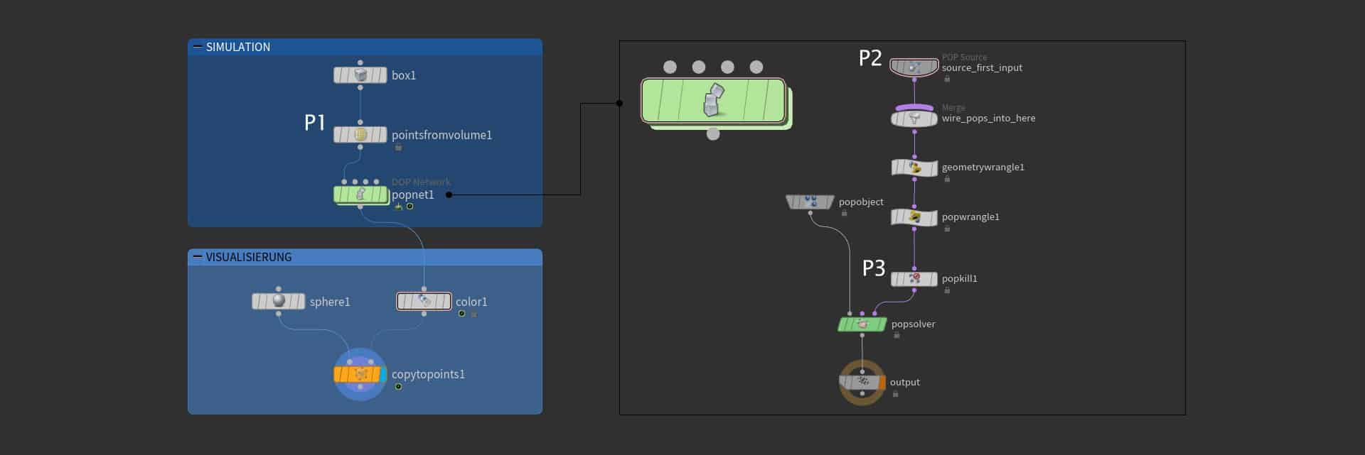
The POP network has only been described to some extent, but it is certainly helpful to know the parameter values and the entire structure of the network. To create the points, a box SOP measuring 20 m x 20 m x 20 m is connected to a Points From Volume SOP in a Geometry OBJ. The size of the box is of course not limited to the above values.

The tags P1, P2 and P3 can be seen in the network diagram. These designations stand for the parameter settings of the corresponding node in the following table:
| P1 | P2 | P3 | |||
| Point Separation | 1 | Source > Emisson Type | Points | Size X | ch(“../../box1/sizex”) |
| Jitter Seed | 1.5 | Source > Geometry Source | Use First… | Size Y | ch(“../../box1/sizey”) |
| Jitter Scale | 1.5 | Birth > Const. Birth Rate | 250 | Size Z | ch(“../../box1/sizez”) |
| Birth > Life Expectancy | 50 | Centre X | ch(“../../box1/tx”) | ||
| Birth > Life Variance | 20 | Centre Y | ch(“../../box1/ty”) | ||
| Centre Z | ch(“../../box1/tz”) | ||||
| Invert | ON |


