Blergh! Word Art! In Houdini?

Houdini can read in external data in various ways. The most comprehensive is certainly a self-written Python parser, but that is not necessary here, because Houdini comes with the Table Import Node as standard. This makes it possible to import tables in CSV format. If you look under the bonnet of the table import node, you will of course find a Python script there anyway. This is one of the reasons why I like Houdini so much: almost everything is open and can be studied or adapted to your own needs.

Import

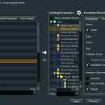
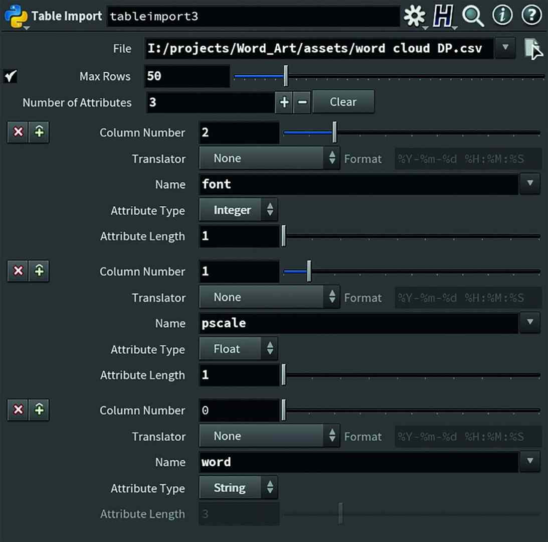
The CSV format contains values that are separated by commas (CSV = comma separated values). These can be words or numbers. Most spreadsheet programmes can save or export tables as CSV. I use Google Sheets here, and it works great: the table import node initially only creates points, which then contain these values in attributes. I use the attributes:

@word, @pscale, @font.

@word gets the values from column A, which is the first column. In Houdini, counting usually starts with zero, hence Column Number 0. The attribute type is a string.

@pscale is a special attribute specified by Houdini. @pscale stands for Point Scale, i.e. the size of a point. This is Column Number 1, and the type in this case is a float, i.e. a floating point number. I could therefore also have entered 1.5 or 2.3 as values in the table.

i have defined @font as type integer, i.e. as an integer. As I want to use three different fonts, I have entered 0, 1 or 2 as values in the table.

The Table Import can also translate (e.g. Lat/Long to Sphere), but the Translator is not needed here.

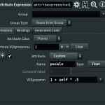
The second node is Enumerate. This creates an @index attribute with which the points are counted in order to be able to assign them later. The group type must be changed from “Primitives” to “Points”. The next two nodes are not absolutely necessary, but as I wanted to create other sizes and these should be somewhat random, I first used Attribute Expression to convert the @pscale values 1,2,3 into 1.5, 2 and 2.5. To do this, “Custom” must be entered in the node attribute and “pscale” as the name and “Float” for the type. I use the VEXpression for this: “1 self * .5”.
And of course, I could have entered these values in the table straight away, but I didn’t. The zero named here as “OUT_points_with_attributes” is not necessary for the function, but is part of good style.

Loop it!

Now the first loop comes into play. This is a For Each Point loop. It contains 3 font nodes, one for each font. Firstly, I created a font node for this and added the spare input required later. To do this, click on the cogwheel and select “Add Spare Input”.

This font node was then referenced twice using drag-and-drop with the Shift, Ctrl and Alt keys held down. For the copies, I then held down the Shift and Ctrl keys and clicked on Font to remove the reference link. Alternatively, this can also be done with the right mouse button menu and “Delete Channels”.

Fonts

The most important node when it comes to text is of course the font node. It can generate both polygons and Bezier curves or both at the same time. I use polygons here. I have set the level of detail to 4 so that the tessellation is nice and fine.

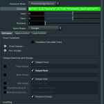
Working with Bezier curves is also great, but unfortunately not useful here, as the UV layout node used later cannot process them. Now it gets a little more magical or technical. In the “Spare Input0” parameter, the “../foreach_begin1” node is referenced by drag-and-drop or, if you want and like typing, you can do that too. The text to be created is normally simply entered in the text field, but we want to read it in from the CSV table, which has already been converted into points. Backticks can be used here to execute code.

The command required here is “points”, whereby it is not about several points, but about string values from points. The “s” at the end stands for “string”. The first spare input is addressed with “-1”. The zero after it is the first point, here it is always just one point anyway, as we are looping over the points. Then “word”, because we want to read the @word attribute. Brackets around it and a backtick and that’s it.

As an aside and for the sake of completeness, “Add Text Attributes” should also be mentioned here. It is not needed here, but is very cool for other text gimmicks. If the box is ticked, the attributes @textindex, which indicates the number of letters in the word, and @textsymbol, which indicates which letter it is, are created for each letter or primitive. However, this is an ASCII value, i.e. a number. “f”, for example, is then 102.

The three font nodes are then connected with a switch that reads the @font attribute. I have also created a spare input for this. This time it is the “point” command and not “points”, as only a number is read out here and not a string. So “point(-1,0, “font”,0)”. In this case, “-1” is again the spare input, “0” is the first point, “font” is the attribute and the last “0” is a necessary argument, which doesn’t really make sense here. However, if we wanted to read out a vector, “0” would be X, “1” would be Y and “2” would be Z. This is also only mentioned here for the sake of completeness.

Copy to points

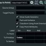
Okay, Houdini! Now we come to the copy to points node. First of all, some information in passing: This node will change a lot in H18 and make actions like this easier. No matter. Pack and Instance is not needed here. Transform Using Point Orientation is also not required here, but can also be on. Copy Points Attributes is used because we still need @index. So enter “index” under Set/To Primitive. Delete everything else.

Now you should be able to see a bunch of fonts on top of each other. Before, there was nothing to see in the viewport except a dot in the centre, at most. Tip: In the “foreach_end1” node you can set to “Single Pass” for debugging, then only one iteration of the loop is executed. And always keep an eye on the geometry spreadsheet, where you can see the values of attributes.
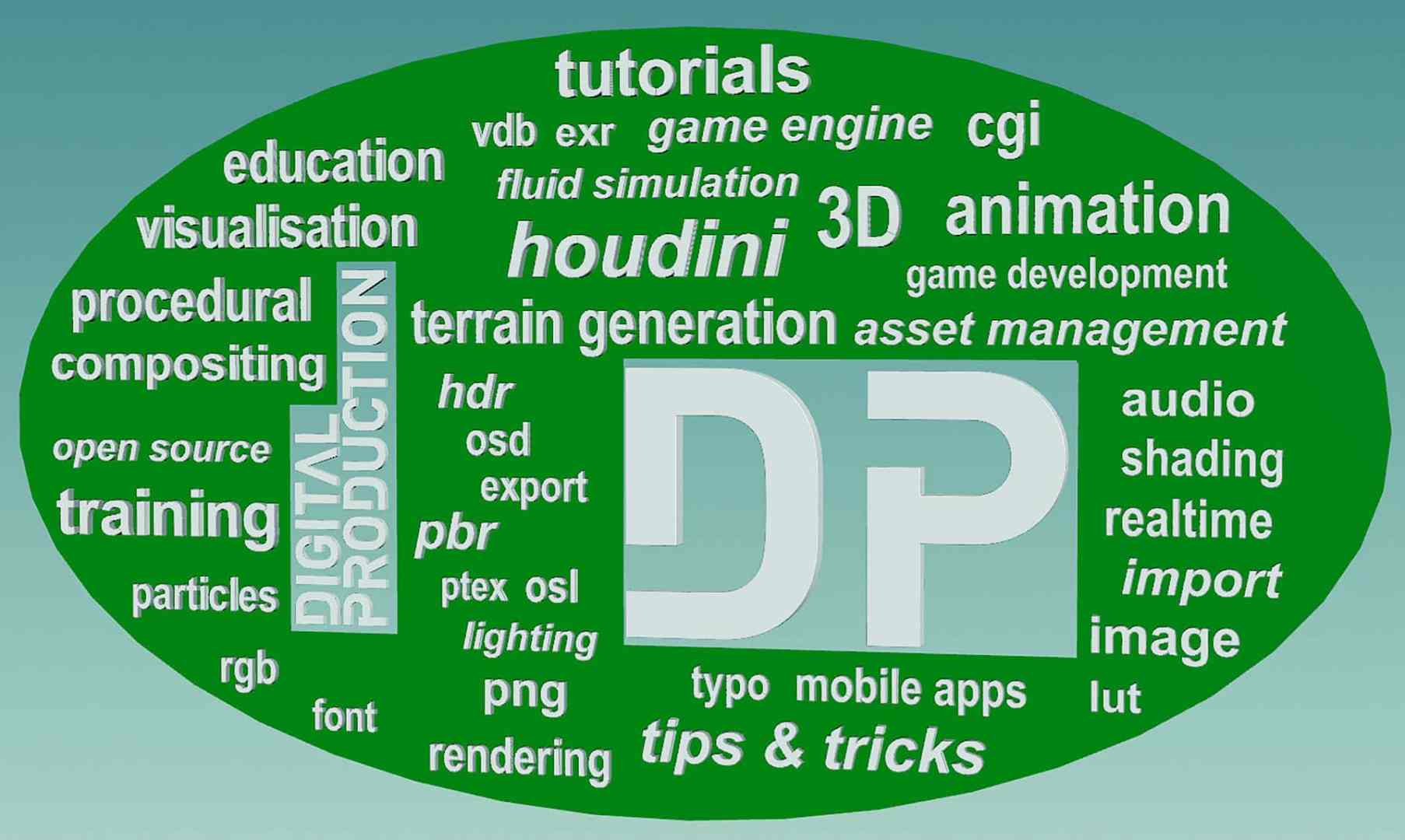
Now we come to the UV layout node, which is used here to distribute the words in a shape. In the picture, I have coloured the shape green. I have left space for the two logos of DP and DIGITAL PRODUCTION. Connecting this shape to the second input of the UV layout node should not be too complex. Of course, the words with the @index attribute go into the first one.

UVs

The UV layout node normally uses the @island attribute to delimit the UV parts from each other and the @uv attribute for the positions of the vertices on the UV map. Since there are no UV coordinates here at all, we replace “uv” twice with “P”.

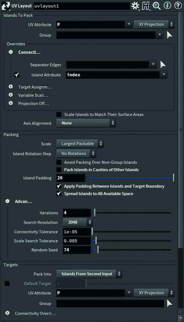
in Houdini, @P is the position of the vertices. For Axis Alignment we select “none” and for Island Rotation Step we set “No Rotations”. If you want to create a Word Cloud with rotated words, they should either be rotated beforehand or you should select 90°, for example, so that no words are upside down.

Padding is the distance between the shapes to be distributed, in this case words, and Scale should be set to “Largest Packable”. The “Advan…” settings are also interesting. This must stand for Advanced. There are iterations here. Here the node randomly tries different layouts and then uses the layout with the best space utilisation. However, each iteration takes time, and 4 is sufficient for this purpose. Different layout versions can be generated with “Random Seed”.
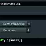
That’s it as far as the layout is concerned, but now we want it in 3D. To switch to a so-called Packed Workflow, we need an @name attribute with a string, i.e. text content. At the moment, we only have an @index attribute, and these are numbers. We do this with an attribute wrangle node.

Select “Primitives” under Run Over and enter the following VEXpression: “s@name = sprintf(“%d”, i@index);”. This creates an @name attribute, which then contains the number as a string. For more details on this VEX function, please refer to the Houdini documentation, which would go beyond the scope of this article.

Now the whole thing is packed, i.e. each word is now represented by a point. This is practical because it is now easier to select the words, for example, in order to make manual corrections to the positions. Simply use an Edit Node to do this.

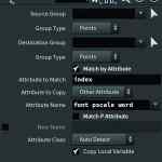
Before or after the edit node, I used an attribute copy node to write the attributes from the beginning @font, @pscale, @word back to the points, which now contain the packed geometry. Again, @index is used to assign the source and target points (Attribute to Match). Only @pscale is actually needed, but never mind. If you want, you could customise this even more variably and select words more easily or, for example, extrude them differently depending on the font.
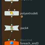
Now rotate another loop and extrude the words. To do this, create a For-Each Primtive Loop and place an Unpack followed by a Pack Node. A polyextrude is placed in between.

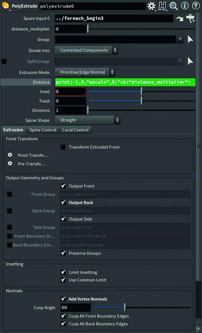
Then either drag and drop the “foreach_begin3” into the spare input created or enter “../foreach_begin3”. I have set the parameter “distance_multiplier” to 0.025.
The magic is in the Distance parameter; enter “point(-1,0, “pscale”,0)*ch(“distance_multiplier”)” enter. Now @pscale is used to control the thickness of the letters. Do not forget to tick the “Output Back” box, otherwise the letter will be open at the back.

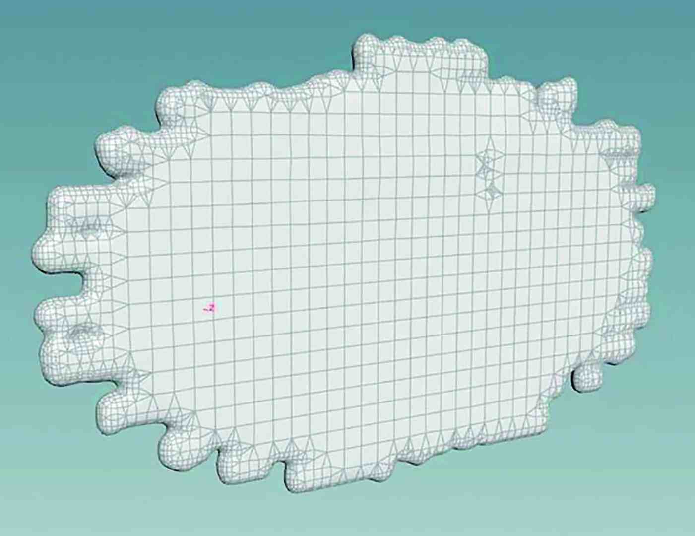
Finally, a file node to save the geometry. It can then be integrated into the rendering scene. The outline plate behind the words was also created procedurally, unfortunately no longer part of this article. But this much can be revealed: I converted a geo into a volume, more precisely into an SDF/VDB. Then enlarged it as an SDF or made it thicker. Then “vdbsmooth” and converted it into a mesh. An Intersection Aanalysis followed by Polypath, then Resample, then Fit and Resample again, and the outline is ready.

Outlook

I would also have liked to have written something about splines, i.e. curve modelling and editing. This works very well in Houdini, even if it takes some getting used to. I would also have liked to discuss rounded edges. But I ran out of pages – we’ll just do that in one of the next issues.